1. Type of Data

• NumPy Array:
  • Homogeneous: All elements must be of the same data type (e.g., integers, floats).
  • This ensures consistency and efficient memory usage.

• List:
  • Heterogeneous: Can contain elements of different types (e.g., integers, strings, other lists).

2. Performance

• NumPy Array:
  • Faster for numerical computations because they are implemented in C and use contiguous memory.
  • Supports vectorized operations (e.g., performing operations on the entire array without loops).

• List:
  • Slower, especially for numerical operations, because each element is an object, and Python's dynamic typing adds overhead.
  • Operations typically require loops or explicit handling.

3. Memory Usage

• NumPy Array:
  • More memory-efficient due to fixed-type storage.
  • Uses a single block of memory for all elements.

• List:
  • Less memory-efficient since each element is a full Python object with type and other metadata.

4. Functionality

• NumPy Array:
  • Supports mathematical operations like addition, subtraction, matrix multiplication, etc., directly.
  • Provides numerous built-in functions for statistical, mathematical, and linear algebra operations.

• List:
  • Limited mathematical functionality; operations like addition or multiplication are not inherently mathematical (e.g., [1, 2] + [3, 4] results in [1, 2, 3, 4]).

5. Dimensionality

• NumPy Array:
  • Can be multi-dimensional (1D, 2D, 3D, etc.).
  • Ideal for working with matrices, tensors, or high-dimensional data.

• List:
  • Can be nested to create "multi-dimensional" lists, but handling them is less intuitive and less efficient than with NumPy arrays.

6. Mutability

• NumPy Array:
  • Mutable, but with constraints: You can't change the size of the array, though you can modify the elements.

• List:
  • Fully mutable: You can add, remove, or modify elements freely.

7. Indexing

• NumPy Array:
  • More advanced slicing and indexing capabilities (e.g., boolean indexing, broadcasting).

• List:
  • Basic slicing and indexing are supported, but without the advanced features of NumPy.

8. Use Cases

• NumPy Array:
  • Ideal for scientific computing, numerical analysis, and data manipulation.

• List:
  • Better for general-purpose programming where flexibility and mixed data types are required.

Create a NumPy ndarray Object

import numpy as np

arr = np.array([1, 2, 3, 4, 5])

print(arr)

print(type(arr))

#We can create a NumPy ndarray object by using the array() function.

0-D Arrays

arr = np.array(42)
#Create a 0-D array with value 42

2-D Arrays

arr = np.array([[1, 2, 3], [4, 5, 6]])
#Create a 2-D array containing two arrays with the values 1,2,3 and 4,5,6:

3-D arrays

arr = np.array([[[1, 2, 3], [4, 5, 6]], [[1, 2, 3], [4, 5, 6]]])
#Create a 3-D array with two 2-D arrays, both containing two arrays with the values 1,2,3 and 4,5,6:

Check Number of Dimensions?

a = np.array(42)
b = np.array([1, 2, 3, 4, 5])
c = np.array([[1, 2, 3], [4, 5, 6]])
d = np.array([[[1, 2, 3], [4, 5, 6]], [[1, 2, 3], [4, 5, 6]]])

print(a.ndim)
print(b.ndim)
print(c.ndim)
print(d.ndim)

Higher Dimensional Arrays

arr = np.array([1, 2, 3, 4], ndmin=5)
#Create an array with 5 dimensions and verify that it has 5 dimensions:

Access Array Elements

arr = np.array([1, 2, 3, 4])

print(arr[0])

#Get the first element from the following array

#Access the element on the first row, second column:

arr = np.array([[1,2,3,4,5], [6,7,8,9,10]])

print('2nd element on 1st row: ', arr[0, 1])

#Access the third element of the second array of the first array:


arr = np.array([[[1, 2, 3], [4, 5, 6]], [[7, 8, 9], [10, 11, 12]]])

print(arr[0, 1, 2])

Negative Indexing

#Print the last element from the 2nd dim:


arr = np.array([[1,2,3,4,5], [6,7,8,9,10]])

print('Last element from 2nd dim: ', arr[1, -1])

Slicing arrays

#Slice elements from index 1 to index 5 from the following array:

arr = np.array([1, 2, 3, 4, 5, 6, 7])

print(arr[1:5])

#Slice elements from index 4 to the end of the array:

print(arr[4:])

#Slice elements from the beginning to index 4 (not included):

print(arr[:4])

#Slice from the index 3 from the end to index 1 from the end:

print(arr[-3:-1])

#Return every other element from index 1 to index 5:

print(arr[1:5:2])

Slicing 2-D Arrays

#From the second element, slice elements from index 1 to index 4 (not included):

arr = np.array([[1, 2, 3, 4, 5], [6, 7, 8, 9, 10]])

print(arr[1, 1:4])

#From both elements, return index 2:

print(arr[0:2, 2])

#From both elements, slice index 1 to index 4 (not included), this will return a 2-D array:

print(arr[0:2, 1:4])

The Difference Between Copy and View

The main difference between a copy and a view of an array is that the copy is a new array, and the view is just a view of the original array.

The copy owns the data and any changes made to the copy will not affect original array, and any changes made to the original array will not affect the copy.

The view does not own the data and any changes made to the view will affect the original array, and any changes made to the original array will affect the view.

COPY:

#Make a copy, change the original array, and display both arrays:

arr = np.array([1, 2, 3, 4, 5])
x = arr.copy()
arr[0] = 42

print(arr)
print(x)

VIEW:

#Make a view, change the original array, and display both arrays:

arr = np.array([1, 2, 3, 4, 5])
x = arr.view()
arr[0] = 42

print(arr)
print(x)

NumPy arrays have an attribute called shape that returns a tuple with each index having the number of corresponding elements.

#Print the shape of a 2-D array:

arr = np.array([[1, 2, 3, 4], [5, 6, 7, 8]])

print(arr.shape)
#The example above returns (2, 4), which means that the array has 2 dimensions, where the first dimension has 2 elements and the second has 4.

Reshaping arrays

Reshaping means changing the shape of an array.

The shape of an array is the number of elements in each dimension.

By reshaping we can add or remove dimensions or change number of elements in each dimension.

Reshape From 1-D to 2-D

#Convert the following 1-D array with 12 elements into a 2-D array.
#The outermost dimension will have 4 arrays, each with 3 elements:

arr = np.array([1, 2, 3, 4, 5, 6, 7, 8, 9, 10, 11, 12])

newarr = arr.reshape(4, 3)

print(newarr)

Reshape From 1-D to 3-D

#Convert the following 1-D array with 12 elements into a 3-D array.
#The outermost dimension will have 2 arrays that contains 3 arrays, each with 2 elements:

arr = np.array([1, 2, 3, 4, 5, 6, 7, 8, 9, 10, 11, 12])

newarr = arr.reshape(2, 3, 2)

print(newarr)

Unknown Dimension

You are allowed to have one "unknown" dimension.

Meaning that you do not have to specify an exact number for one of the dimensions in the reshape method.

Pass -1 as the value, and NumPy will calculate this number for you.

#Convert 1D array with 8 elements to 3D array with 2x2 elements:

arr = np.array([1, 2, 3, 4, 5, 6, 7, 8])

newarr = arr.reshape(2, 2, -1)

print(newarr)

Flattening the arrays

Flattening array means converting a multidimensional array into a 1D array.

We can use reshape(-1) to do this.

arr = np.array([[1, 2, 3], [4, 5, 6]])

newarr = arr.reshape(-1)

print(newarr)

Iterating 3-D Arrays

arr = np.array([[[1, 2, 3], [4, 5, 6]], [[7, 8, 9], [10, 11, 12]]])

for x in arr:
  for y in x:
    for z in y:
      print(z)

Iterating Arrays Using nditer()

The function nditer() is a helping function that can be used from very basic to very advanced iterations. It solves some basic issues which we face in iteration, lets go through it with examples.

arr = np.array([[[1, 2], [3, 4]], [[5, 6], [7, 8]]])

for x in np.nditer(arr):
  print(x)

Iterating With Different Step Size

arr = np.array([[1, 2, 3, 4], [5, 6, 7, 8]])

for x in np.nditer(arr[:, ::2]):
  print(x)

Enumerated Iteration Using ndenumerate()

Enumeration means mentioning sequence number of somethings one by one.

Sometimes we require corresponding index of the element while iterating, the ndenumerate() method can be used for those usecases.

#Enumerate on following 1D arrays elements

arr = np.array([1, 2, 3])

for idx, x in np.ndenumerate(arr):
  print(idx, x)

#Enumerate on following 2D array's elements:
arr = np.array([[1, 2, 3, 4], [5, 6, 7, 8]])

for idx, x in np.ndenumerate(arr):
  print(idx, x)

Generate a random number

x = random.randint(100)
#Generate a random integer from 0 to 100:

Generate a random float

x= random.rand()
#The random module's rand() method returns a random float between 0 and 1.

Generate a random array

x=random.randint(100, size=(5)) # 1-D array
x = random.randint(100, size=(3, 5)) # 2-D array
#The randint() method takes a size parameter where you can specify the shape of an array.

Generate a random float array

x= random.rand(3) #1-D array
x= random.rand(3,5) #2-D array

Generate Random Number From Array

#The choice() method allows you to generate a random value based on an array of values.
#The choice() method takes an array as a parameter and randomly returns one of the values.
x = random.choice([3, 5, 7, 9])

x = random.choice([3, 5, 7, 9], size=(3, 5))
#Generate a 2-D array that consists of the values in the array parameter (3, 5, 7, and 9)

Random Distribution

""" 
Generate a 1-D array containing 100 values, where each value has to be 3, 5, 7 or 9.

The probability for the value to be 3 is set to be 0.1

The probability for the value to be 5 is set to be 0.3

The probability for the value to be 7 is set to be 0.6

The probability for the value to be 9 is set to be 0
"""
x = random.choice([3, 5, 7, 9], p=[0.1, 0.3, 0.6, 0.0], size=(100))

Random Permutations

arr = np.array([1, 2, 3, 4, 5])

random.shuffle(arr)
#The shuffle() method makes changes to the original array.

arr = np.array([1, 2, 3, 4, 5])

print(random.permutation(arr))

#The permutation() method returns a re-arranged array (and leaves the original array un-changed).

Seaborn

Visualize Distributions With Seaborn

Seaborn is a library that uses Matplotlib underneath to plot graphs. It will be used to visualize random distributions.

Plotting a Distplot

import matplotlib.pyplot as plt
import seaborn as sns

sns.distplot([0, 1, 2, 3, 4, 5])

#sns.distplot([0, 1, 2, 3, 4, 5], hist=False) -> plot without the Histogram

plt.show()

Normal (Gaussian) Distribution

loc - (Mean) where the peak of the bell exists.

scale - (Standard Deviation) how flat the graph distribution should be.

size - The shape of the returned array.

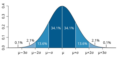
x = random.normal(loc=1, scale=2, size=(2, 3))
#Generate a random normal distribution of size 2x3 with mean at 1 and standard deviation of 2

Visualization of Normal Distribution

from numpy import random
import matplotlib.pyplot as plt
import seaborn as sns

sns.distplot(random.normal(size=1000), hist=False)

plt.show()

Binomial Distribution

Binomial Distribution is a Discrete Distribution.

It describes the outcome of binary scenarios, e.g. toss of a coin, it will either be head or tails.

It has three parameters:

n - number of trials.

p - probability of occurence of each trial (e.g. for toss of a coin 0.5 each).

size - The shape of the returned array.

from numpy import random

x = random.binomial(n=10, p=0.5, size=10)

print(x)

#Given 10 trials for coin toss generate 10 data points:

Probability mass function

If the random variable X follows the binomial distribution with parameters n ∈ N and p ∈ [0, 1], we write X ~ B(n, p). The probability of getting exactly k successes in n independent Bernoulli trials (with the same rate p) is given by the probability mass function:

for k = 0, 1, 2, ..., n, where

Uniform Distribution

Used to describe probability where every event has equal chances of occuring.

E.g. Generation of random numbers.

It has three parameters:

low - lower bound - default 0 .0.

high - upper bound - default 1.0.

size - The shape of the returned array.

x = random.uniform(size=(2, 3))

print(x)

# plotting

sns.distplot(random.uniform(size=1000), hist=False)

plt.show() 

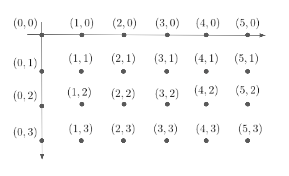
numpy.meshgrid: Detailed Explanation

The numpy.meshgrid function is a powerful utility in NumPy for generating coordinate grids, which are commonly used in mathematical computations, visualizations, and simulations. Here’s a detailed breakdown of its functionality, usage, and common scenarios.

Purpose of numpy.meshgrid

The primary purpose of numpy.meshgrid is to create coordinate matrices from coordinate vectors. Given one-dimensional arrays (or vectors) that define the axes of a grid, meshgrid expands these arrays into multidimensional grid representations. These grids are useful for evaluating functions over a grid of points or plotting 2D and 3D surfaces.

Function Signature

numpy.meshgrid(*xi, copy=True, sparse=False, indexing='xy')

Parameters:

1. xi (array_like):
   • One-dimensional arrays representing the coordinates of the grid points along each axis.
   • You can provide two or more input arrays, depending on the dimensionality of the grid you need.

2. copy (bool, optional):
   • If True (default), the output arrays are copies of the original arrays.
   • If False, the function may return views to the original data (saves memory).

3. sparse (bool, optional):
   • If False (default), the full grid arrays are created.
   • If True, sparse grids are generated to save memory. This is particularly useful for computations that don’t require a full grid.

4. indexing (str, optional):
   • Controls the indexing convention.
     • 'xy': Cartesian indexing (default).
     • 'ij': Matrix indexing.

Returns:

• A list of N arrays, where N is the number of input arrays. Each array has the same shape, representing the grid coordinates.

Key Concepts

1. Cartesian vs. Matrix Indexing

• 'xy' indexing assumes the first input array corresponds to the x-coordinates, and the second to y-coordinates. This is intuitive for plotting in Cartesian systems.

• 'ij' indexing assumes matrix-style indexing, where the first input array corresponds to rows (i.e., y-coordinates), and the second to columns (i.e., x-coordinates).

2. Full vs. Sparse Grids

• Full grids explicitly represent every grid point and are useful for visualizations.

• Sparse grids represent only the unique coordinates needed to define the grid, saving memory for large computations.

Examples

Example 1: Basic Cartesian Grid

import numpy as np

x = np.array([1, 2, 3])
y = np.array([4, 5])

X, Y = np.meshgrid(x, y, indexing='xy')

print("X:\\n", X)
print("Y:\\n", Y)

Output:

X:
 [[1 2 3]
  [1 2 3]]
Y:
 [[4 4 4]
  [5 5 5]]

Here, X contains copies of the x-coordinates for each row, and Y contains copies of the y-coordinates for each column.

Example 2: Sparse Grid

X, Y = np.meshgrid(x, y, sparse=True)

print("X:\\n", X)
print("Y:\\n", Y)

Output:

X:
 [[1 2 3]]
Y:
 [[4]
  [5]]

The sparse grid avoids redundant storage of data.

Example 3: Matrix Indexing

X, Y = np.meshgrid(x, y, indexing='ij')

print("X:\\n", X)
print("Y:\\n", Y)

Output:

X:
 [[1 1 1]
  [2 2 2]
  [3 3 3]]
Y:
 [[4 5 6]
  [4 5 6]
  [4 5 6]]

Matrix indexing swaps the role of rows and columns.

Example 4: 3D Grid

z = np.array([7, 8])
X, Y, Z = np.meshgrid(x, y, z, indexing='xy')

print("X:\\n", X)
print("Y:\\n", Y)
print("Z:\\n", Z)

Output:

X:
 [[[1 1]
   [1 1]]

  [[2 2]
   [2 2]]

  [[3 3]
   [3 3]]]
Y:
 [[[4 4]
   [5 5]]

  [[4 4]
   [5 5]]

  [[4 4]
   [5 5]]]
Z:
 [[[7 8]
   [7 8]]

  [[7 8]
   [7 8]]

  [[7 8]
   [7 8]]]

Here, X, Y, and Z represent the grid coordinates in 3D space. Each slice of the arrays corresponds to a fixed value of one axis, while the other two vary.

Use Cases

1. Plotting 2D and 3D surfaces:
   • Grids generated by meshgrid are used to evaluate functions and plot surfaces in libraries like Matplotlib.

   import matplotlib.pyplot as plt
   from mpl_toolkits.mplot3d import Axes3D
   
   x = np.linspace(-5, 5, 50)
   y = np.linspace(-5, 5, 50)
   X, Y = np.meshgrid(x, y)
   Z = np.sin(np.sqrt(X**2 + Y**2))
   
   fig = plt.figure()
   ax = fig.add_subplot(111, projection='3d')
   ax.plot_surface(X, Y, Z, cmap='viridis')
   plt.show()
   

2. Numerical simulations:
   • Used in finite element methods or solving partial differential equations.

3. Vectorized computations:
   • Grids allow for efficient computations over large datasets without explicit loops.

4. Image Processing:
   • Grids of coordinates are useful for operations like transformations or sampling.

Best Practices

• Use sparse grids (sparse=True) for computations that don’t require the full grid structure, to save memory.

• Choose appropriate indexing (xy or ij) based on the specific problem domain (e.g., plotting vs. matrix computations).

• Leverage broadcasting with sparse grids to further optimize memory usage.

Common Pitfalls

1. Memory Usage:
   • Generating large grids can consume significant memory, especially in 3D or higher dimensions. Use sparse grids when possible.

2. Indexing Confusion:
   • Be cautious about the difference between 'xy' and 'ij' indexing, as it can lead to subtle bugs in applications.

Summary

numpy.meshgrid is an essential tool for creating coordinate grids. Whether for visualizations, numerical simulations, or general computational tasks, understanding its parameters and options allows for efficient and flexible grid generation.